ggplot2

Pair-programming activity

Before you start

Work in pairs, one laptop. The driver types. The navigator reads the task aloud and says what to type. Swap at every Swap.

Grey boxes are live R. Edit, then Run Code. The first run takes a few seconds.

Based on Wickham, Çetinkaya-Rundel & Grolemund, R for Data Science (2e), ch. 1.

1. The data

Column	What it is
species	Adelie, Chinstrap or Gentoo
island	Biscoe, Dream or Torgersen
bill_length_mm, bill_depth_mm	bill size
flipper_length_mm	flipper length
body_mass_g	body mass
sex, year	sex and year observed

Your turn. How many rows and columns does penguins have?

Solution:

dim(penguins)

344 rows (penguins), 8 columns (variables).

2. The goal

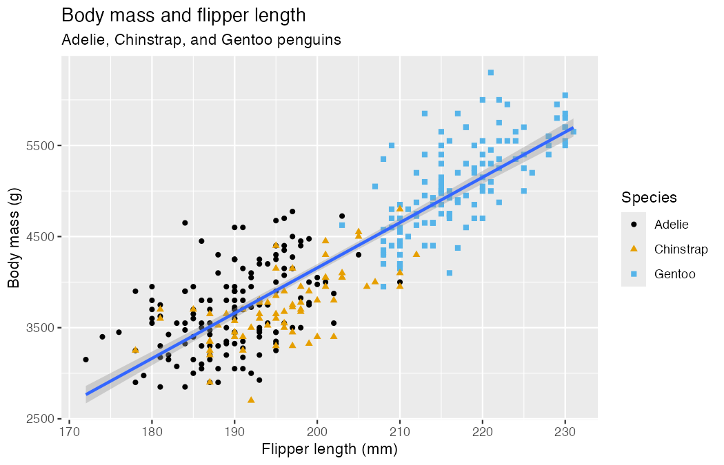
By the end of section 3 you will have rebuilt this plot.

3. Build a plot, layer by layer

Every ggplot has three parts:

ggplot(data = <DATA>, mapping = aes(<MAPPINGS>)) +
  <GEOM_FUNCTION>()

Step 1 — data. An empty canvas.

Step 2 — mapping. aes() links columns to axes.

Step 3 — geom. How to draw each row.

Talk it over. Describe the relationship in one sentence. The warning mentions 2 rows — why?

Solution

Heavier penguins have longer flippers: a strong positive relationship. Two penguins have no flipper length or body mass recorded (NA), so they cannot be plotted.

Step 4 — color. Map a third variable.

Step 5 — a second layer. Add a trend line.

Talk it over. Why three lines? The goal has one.

Solution

color = species sits in ggplot(), so it applies to every layer, and geom_smooth() fits one line per species.

Mappings in ggplot() apply to every layer. Mappings inside a geom apply to that layer only.

Swap

Your turn. Finish the goal plot: add shape = species, labels with labs(), and the colorblind-safe palette scale_color_colorblind() (from ggthemes).

Solution:

library(ggthemes)
ggplot(
  data = penguins,
  mapping = aes(x = flipper_length_mm, y = body_mass_g)
) +
  geom_point(mapping = aes(color = species, shape = species)) +
  geom_smooth(method = "lm") +
  labs(
    title = "Body mass and flipper length",
    subtitle = "Adelie, Chinstrap, and Gentoo penguins",
    x = "Flipper length (mm)", y = "Body mass (g)",
    color = "Species", shape = "Species"
  ) +
  scale_color_colorblind()

Your turn. Plot bill_depth_mm (y) against bill_length_mm (x). Describe what you see.

Solution:

ggplot(penguins, aes(x = bill_length_mm, y = bill_depth_mm)) +
  geom_point()

Overall, a weak negative trend — until you color by species (section 5).

Your turn. This errors. Why? Fix it.

Hint

What should go on the x and y axes?

Solution:

geom_point() needs x and y. Add a mapping:

ggplot(
  data = penguins,
  mapping = aes(x = flipper_length_mm, y = body_mass_g)
) +
  geom_point()

Predict first, then run. What will this look like?

Solution:

Points colored by island, one smooth curve per island (color is global), no grey confidence band (se = FALSE).

Shorter code

The first two arguments are always data and mapping, so you can drop their names:

ggplot(penguins, aes(x = flipper_length_mm, y = body_mass_g)) +
  geom_point()

4. One variable: distributions

Swap

Categorical → bar chart.

Order bars by frequency with fct_infreq() (from forcats):

Numerical → histogram. binwidth sets the width of each bar.

Numerical → density. A smoothed histogram.

Your turn. Put species on the y axis. What changes?

Solution:

ggplot(penguins, aes(y = species)) +
  geom_bar()

Horizontal bars. Handy when labels are long.

Your turn. Run both. Which one is useful?

Solution:

color paints the outline; fill paints the inside. For bars, use fill.

Note: "red" sits outside aes() — it is a fixed value, not a mapping to a column.

Your turn. Histogram of carat in the diamonds data (built into ggplot2). Try binwidth values of 1, 0.1 and 0.01. Which shows the most?

Solution:

ggplot(diamonds, aes(x = carat)) +
  geom_histogram(binwidth = 0.01)

At 0.01 you see spikes at round sizes (0.3, 0.5, 1, 1.5, 2 carats). Too wide a bin hides them.

5. Two or more variables: relationships

Swap

Numerical + categorical → boxplot or density.

Two categorical → stacked bars. position = "fill" shows proportions.

Two numerical → scatterplot (section 3).

Three or more → facets. One small panel per category.

Your turn. Back to the bills. Color by species, then facet by species. What does each reveal?

Solution:

ggplot(penguins, aes(x = bill_length_mm, y = bill_depth_mm,
                     color = species)) +
  geom_point() +
  facet_wrap(~species)

Color: three clear clusters. Facets: within each species, longer bills are deeper — the opposite of what the uncolored plot suggested.

Your turn. Two legends appear. Merge them into one titled “Species”.

Hint

Both mapped aesthetics need the same title.

Solution:

ggplot(penguins, aes(x = bill_length_mm, y = bill_depth_mm,
                     color = species, shape = species)) +
  geom_point() +
  labs(color = "Species", shape = "Species")

Talk it over. Run both. Which question does each answer?

Solution:

1. Which species live on each island? (Torgersen: only Adelie.)
2. Which islands does each species live on? (Adelie: all three.)

Swap

Your turn. The mpg data (ggplot2) has car engine size (displ) and highway mileage (hwy). Plot them, then map cyl to color, then to size. Which works better?

Solution:

ggplot(mpg, aes(x = displ, y = hwy, color = cyl)) +
  geom_point()

cyl is numerical, so color becomes a gradient and size a scale. Now try shape = cyl — it fails: shapes only work for categories.

6. Fix the bug

Swap

Each snippet has one mistake.

Solution:

The + must end a line, not start one.

ggplot(penguins, aes(x = body_mass_g)) +
  geom_histogram()

Solution:

ggplot2 layers join with +, not the pipe |>.

ggplot(penguins, aes(x = species, y = body_mass_g)) +
  geom_boxplot()

Solution:

Inside aes(), "blue" is treated as data (a column whose value is the word “blue”), so the points are red with a “blue” legend. Move it outside:

ggplot(penguins, aes(x = flipper_length_mm, y = body_mass_g)) +
  geom_point(color = "blue")

7. Saving (in RStudio)

ggsave() saves the last plot shown:

ggplot(penguins, aes(x = flipper_length_mm, y = body_mass_g)) +
  geom_point()
ggsave(filename = "penguin-plot.png")  # or .pdf, .svg

Recap

You want to show	Geom
counts of a category	geom_bar()
spread of a number	geom_histogram(), geom_density()
number by category	geom_boxplot()
two numbers	geom_point(), geom_smooth()
a third variable	color, shape, size, or facet_wrap()

Mapping (aes(color = species)) uses a column. Setting (color = "blue") uses one value.